ACIC 2026•Poster Session 2•Wed May 13, 2026•Salt Lake City, Utah
SHAP has short memory.
Causal SHAP remembers the DAG.
DAG-informed, expert-augmented Causal SHAP recovers causally-coherent feature importance that standard explainable ML misses.




Poster authors
Aimee Harrison1,Lexi Pasi2,Justin Ross3,Jenny G. Alderden4,Andy Wilson3*
- 1 Navidence
- 2 Lucidity Sciences
- 3 University of Utah
- 4 Boise State University
* Presenter
Introduction: Why explainability, why now
Modern machine-learning (ML) systems have shown remarkable predictive accuracy across many domains, but they tell us what they predicted without telling us why. Clinicians, regulators, and patients reasonably want both. The field of Explainable Artificial Intelligence (XAI) grew up around that gap, building methods that surface a fitted model's internal logic in human-readable form.
XAI methods fall into two broad camps:
- Post hoc explanations attach to an already-trained black box. The most familiar of these is .
- Inherently interpretable models are transparent by construction, and include decision rules and generalized additive models.
In life sciences, an AI explanation needs to be as truthful as we can make it. An explanation that misleads a clinician misleads a treatment plan. In clinical settings, XAI is most often deployed inside embedded in electronic health records. Recent meta-analyses name SHAP as the leading clinician-facing XAI method, while flagging that explanation fidelity, clinician trust, and real-world usability remain underdeveloped (Abbas et al. 2025; El Arab et al. 2025).
In the poster, we explore two case studies of causally-informed XAI: a simulation under a known data-generating process, and an analysis of hospital-acquired pressure injury risk in MIMIC-IV ICU patients. This site serves to expand on those case studies with full methods, interactive figures, and a candid discussion of where the correction earns its keep.
Explainable ML has a structural blind spot
If you have used SHAP, , or before, you have used a method that treats features as if they were exchangeable. The math behind these methods proceeds as though the order in which a model considers features does not matter. But we know that in a causal system, the order does matter. Causes come before effects, and credit for an outcome should flow upstream against the arrows of causation. When an attribution method ignores the underlying causal structure, features that sit close to the outcome in the causal graph tend to absorb credit that belongs further upstream. This misallocation is a .
Concretely: mediators near the outcome accumulate credit they did not generate. Confounders near the treatment may or may not, depending on conditioning. Root causes far from the outcome get under-credited. The artifact is mathematical, not statistical. It is built into any attribution method that averages over all p! feature orderings without regard to direction.
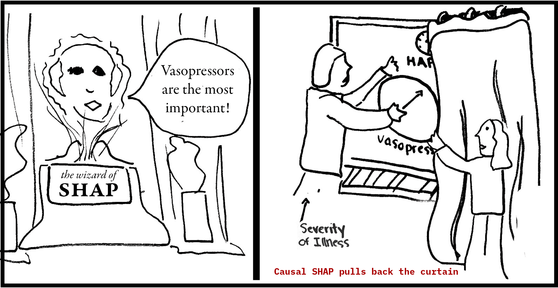
Consider a model that predicts hospital-acquired pressure injury in Intensive Care Unit (ICU) patients. SHAP is run to assess feature importance. The top-ranked SHAP feature comes back as vasopressor use. The straightforward read is that vasopressors are causing pressure injuries. But if you take causality into account, it quickly becomes clear that such an interpretation is wrong. Vasopressors are administered to the sickest, most hemodynamically unstable patients, who are also at the highest risk of pressure injury for many other reasons. The drug here is a marker of severity, not a cause of the outcome.
SHAP isn't lying here. SHAP decomposes a specific fitted model's predictions on specific data points. That is a narrower claim than “SHAP ranks features by how much they predict the outcome,” and narrower still than “SHAP identifies which features cause the outcome.” Two equally-fitting models trained on the same data give different SHAP rankings, because they learn different functional relationships. Two correlated features carrying the same predictive signal can have their credit split arbitrarily between them depending on model internals. Even before causal structure enters the picture, a SHAP value is faithful to one fitted model's internal logic, not to a feature's real-world informativeness.
Why standard SHAP fails
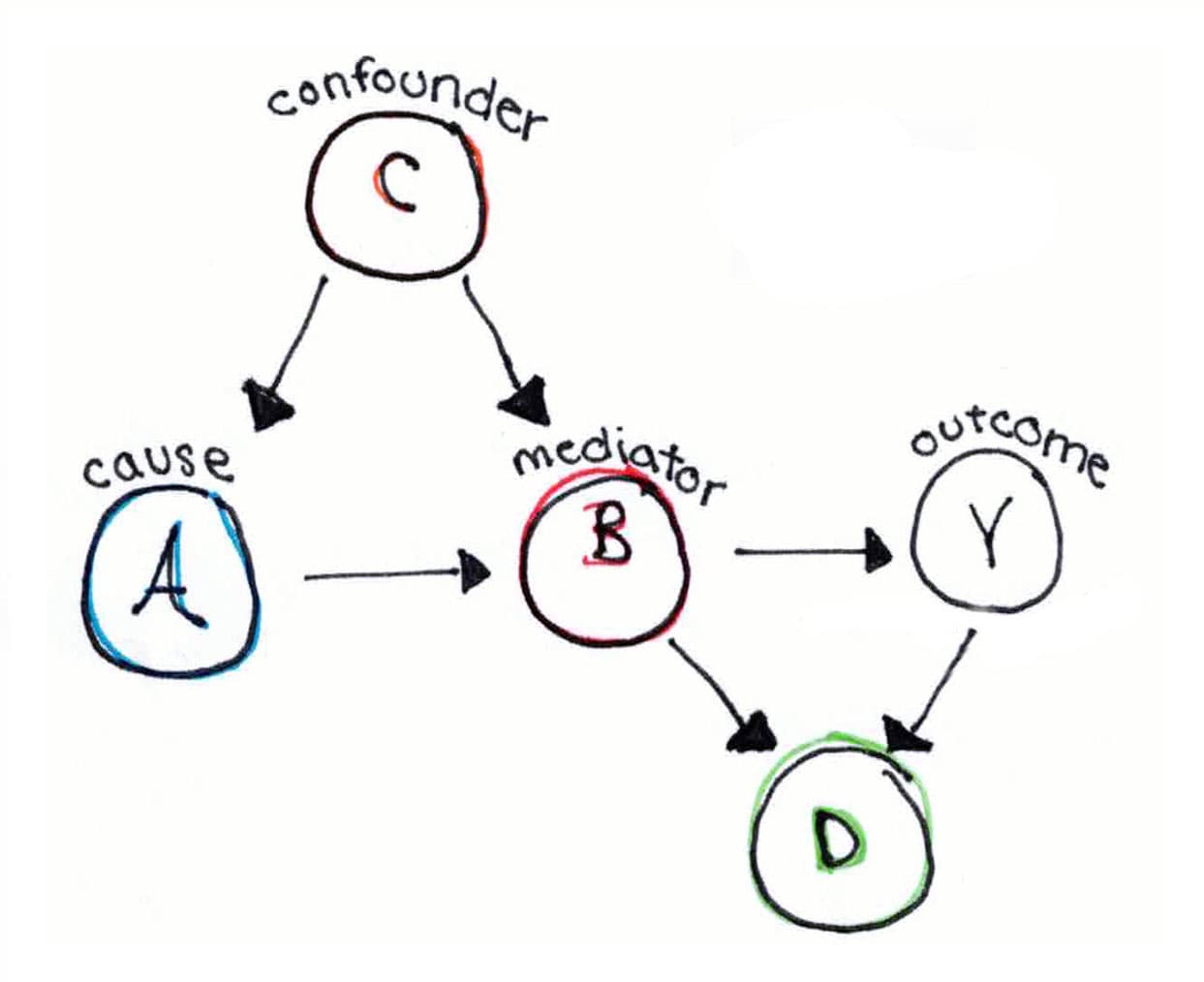
The closer a variable sits to Y, the more credit SHAP gives it (even when it isn't the cause). The two cards below show what that distortion looks like in two canonical small graphs: tap each card to flip between the underlying causal truth and the picture standard SHAP assembles when it ignores that structure.
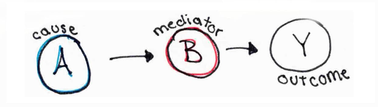
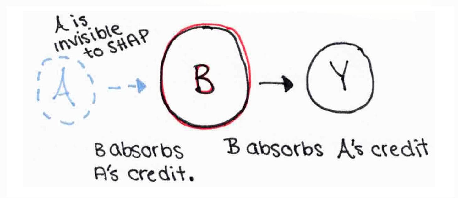
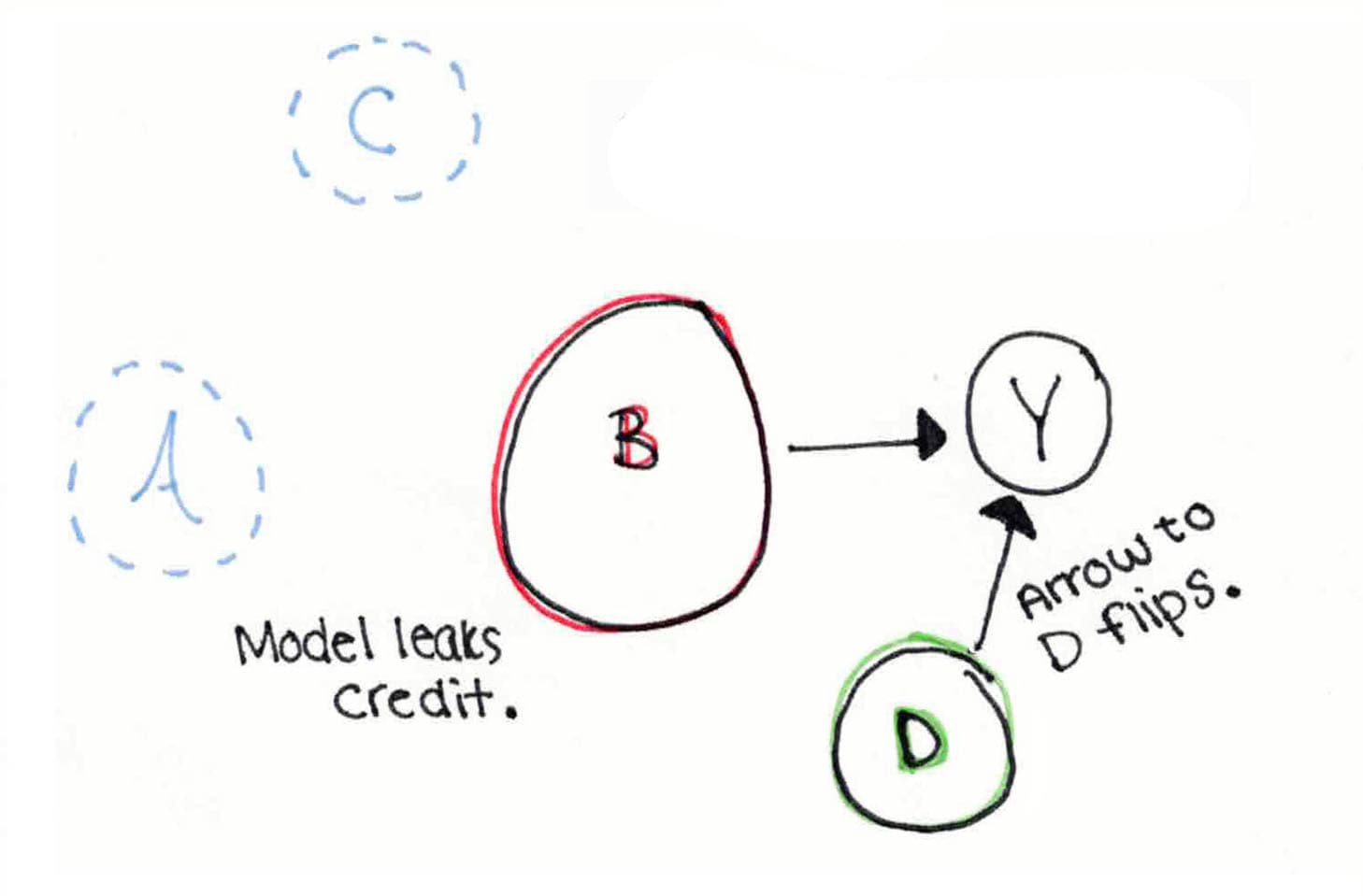
The asks how much credit each feature deserves for a prediction by averaging the feature's marginal contribution across every possible ordering of the features (for features, that is orderings). Each ordering imagines a world in which features arrive sequentially and the model updates its prediction with each arrival. Standard SHAP averages over every possible arrival order, including causally impossible ones. In that average, “Outcome arrives before Treatment” is just as likely as “Treatment arrives before Outcome.”
That is fine when features are exchangeable. It is not fine when features have causal structure.
Imagine a causal DAG for heart failure. We know that blood pressure depends on age, not the other way around. SHAP, however, samples both orderings with equal weight, so it treats “age affects blood pressure” and “blood pressure affects age” as equally likely arrival sequences. The first is structurally plausible. The second is structurally impossible.
The same problem hits . In a causally valid ordering, a mediator must arrive after its parents, since causes precede effects. As a result, mediators tend to land near the end of many orderings. By the time a mediator's turn comes up in the ordering, the model has already incorporated most of the upstream causes, so the marginal contribution it picks up is the part of the prediction not yet explained: the residual. That residual is upstream credit, routed to the mediator. The closer to the outcome a mediator sits, the more residual credit it absorbs.
The problem also extends to . When the feature set includes a downstream descendant of both treatment and outcome, conditioning on it creates a statistical association between treatment and outcome where no causal relationship exists. SHAP, which cannot tell the difference between a causal pathway and a spurious association, credits that path too.
The correction
Heskes et al. (2020) and Janzing et al. (2020) propose a possible correction: compute Shapley values under an rather than an . This is a switch in conditioning, drawing from .
The observational expectation asks what we expect if we observe X at value x. The interventional expectation instead asks what we expect if we intervene to set X to x. The two are equal when X has no upstream causes, but they diverge whenever it does. We discuss a complementary approach in “An alternative path”.
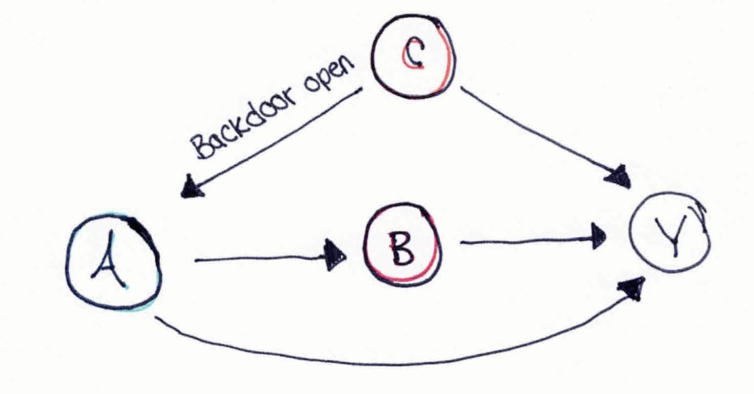
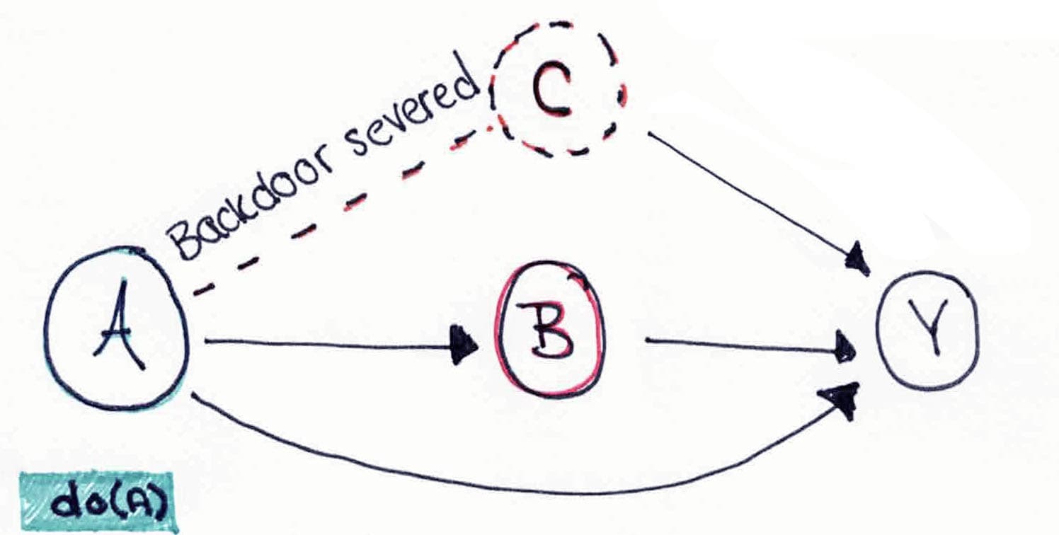
In practice, the corrected algorithm only makes a small set of changes to the standard Shapley computation:
- Restricted permutations. Sampling proceeds only from valid of the DAG, so causes always precede effects and causally impossible orderings are excluded from the average.
- Interventional expectations. When evaluating the model on a partial set of features (a ), features outside the coalition are filled in by sampling from their conditional distribution given their parents in the DAG, rather than from the unconditional marginal. This is what breaks the back-door paths.
- Conditional structural models. For non-root nodes, small surrogate models (typically gradient-boosted regressors) estimate and supply the conditional samples that the interventional step needs.
With these changes in place, credit can no longer flow backward through time or sideways across confounders. Each feature's Shapley contribution is computed along the same pathways the data-generating process actually used.
The Causal SHAP Workflow
Causal SHAP is not an automated pipeline. It is a workflow that asks two kinds of expertise to agree on a single DAG before any attribution is computed: (1) the discovery algorithm contributes statistical evidence; (2) the clinician or epidemiologist contributes domain knowledge. The resolved DAG is something both parties can defend.
Causal discovery alone is insufficient. An epidemiologist knows that demographics precede labs, labs precede vitals, vitals precede interventions, and interventions precede outcomes. That kind of knowledge has to enter the DAG somewhere, because purely data-driven discovery cannot recover it. Our workflow makes that knowledge a first-class input.
Discover
Run a causal-discovery algorithm on observed data to obtain a candidate DAG skeleton.
Run PC, GES, or DirectLiNGAM via causal-learn. The and other constraint-based methods produce a in which some edges are oriented and some remain bidirected, because statistical independence tests cannot distinguish certain from each other. DirectLiNGAM exploits non-Gaussian functional forms in the data to produce a fully directed graph. We typically see only about 20 percent edge agreement between PC and GES on identical inputs, which is part of why expert resolution in Step 2 is essential.
Resolve
A clinician or epidemiologist orients the ambiguous edges using domain knowledge.
The expert orients ambiguous edges using temporal ordering, biological plausibility, and prior trial evidence. dagitty is the standard tool: the expert specifies and visually edits the DAG, then tests the implied conditional independencies against the data. Our app post-processes the adjacency matrix to hard-enforce required and forbidden edges from a domain rule list.
In our simcausal DAG, the clinician is asked questions like: does comorbidity drive treatment, or does treatment create comorbidity? Does inflammation cause hypoxia, or does hypoxia cause inflammation? Does treatment reach outcome directly, or only through mediators? Each answer becomes a required or forbidden edge in the resolved DAG.
Weight
Estimate the strength of each directed edge.
For each directed edge, estimate a mean causal effect via structural equation model coefficients, IDA estimates from pcalg, or a targeted-learning step. Serialize the result to JSON in the format {"Pair": "X1->X2", "Mean_Causal_Effect": 0.63}. This is what fast-causal-shap consumes in Step 4. Linear approximations are exact in linear SEM settings and rough in nonlinear ones.
Compute
Plug the resolved DAG into Causal SHAP and compute attributions.
Install fast-causal-shap, load the JSON edge file with load_causal_strengths(), fit the prediction model, and compute Causal SHAP alongside standard SHAP for comparison. The permutations parameter trades runtime against Monte Carlo accuracy: 50 is fast for screening, 500 is recommended for final reporting.
Sensitivity
Re-run Steps 2 through 4 under alternative plausible DAGs and compare.
A single resolved DAG is one set of structural assumptions. To check robustness, repeat the workflow under several plausible alternatives (forbid an edge, require another, swap a direction) and observe how much the feature attributions move. This is the structural counterpart to probabilistic bias analysis in epidemiology, analogous in spirit to E-values for unmeasured confounding.
Step 2 is where the workflow stops being mechanical. The discovery algorithm hands the clinician a graph it could not finish, and the clinician has to decide which way each unresolved arrow points based on what they know about biology and time.
The interactive panel below stages a miniature version of that moment. The simcausal DAG has three edges the discovery algorithm could not orient. As you choose a direction for each, the bar chart underneath shows how feature attribution rearranges, so you can see the cost of getting an edge wrong and the payoff of getting it right.
Step 2 in miniature
Resolve three edges, watch the attribution settle.
The DAG on the left has three dashed edges the discovery algorithm could not orient. Answer the three questions on the right to set each direction. As you do, the bar chart underneath rearranges in real time.
Resolved DAG
0 of 3 resolved
Dashed = unresolved. Teal = matches the data-generating process. Orange = an alternative orientation.
Resolve each edge
1. Does inflammation cause hypoxia, or does hypoxia cause inflammation?
2. Does CKD drive steroid use, or does steroid use drive CKD?
3. Does steroid reach pressure injury directly, or only through mediators?
Top feature attributions (live)
plain SHAP → Causal SHAP (blend: 0%)
Plain SHAP: mediators and downstream variables hold the top of the ranking. Steroid sits below Inflammation.
Simulation evidence
We first tested the Causal SHAP workflow against synthetic data, where the data-generating process was fully specified. Because the ground-truth causal structure was known, we could measure how well each method recovered it.
Methods
We generated synthetic data using the R package under a known 12-variable DAG with 28 ground-truth directed edges. The data-generating process placed Treatment as the largest causal driver of the outcome. Setting Treatment from 0 to 1 changes Outcome by +11.0 across its direct and mediated paths through Inflammation and Oxygenation. The structural equations and the causal paths relevant to interpretation are below.
We trained a gradient-boosted regression model to predict the outcome from the 11 input features and computed both standard SHAP and causal SHAP on this same fitted model. The methods differ only in which orderings they sample and how they handle absent features when computing coalition values: standard SHAP averages over all 11! feature orderings using observational expectations, while Causal SHAP restricts orderings to those consistent with the known DAG and uses interventional expectations. We compared the resulting rankings to each other, and to the true total causal effects from the structural equations, using Kendall's τ. The headline numbers below come from 50 permutations of the SHAP estimator. We report higher-accuracy comparisons at 500 permutations in the next section.
Results
We ran standard SHAP and Causal SHAP against the synthetic data and compared the two rankings. Two headline statistics summarize the comparison:
Standard SHAP and Causal SHAP disagreed
Kendall's τ between the two rankings was 0.42. With no rank ties, that corresponds to roughly 71% concordant feature pairs—not 42% of pairs agreeing. The methods still rearranged several individual features meaningfully.
- Inflammationmediator#1#1—
- Oxygenationmediator#2#3↓ 1
- Comorbidityupstream#3#5↓ 2
- HRupstream#4#9↓ 5
- Treatmenttreatment#5#4↑ 1
- Ageupstream#6#10↓ 4
- Creatininenull endpoint#7#6↑ 1
- SBPupstream#8#7↑ 1
- BMIupstream#9#8↑ 1
- Glucoseupstream#10#2↑ 8
- Sexupstream#11#11—
- moved toward rank 1
- moved away from rank 1
- unchanged
Ranks are observed results from the 50-permutation run. They are not SHAP magnitudes or effect sizes.
Mediators received different attribution
We compared how much attribution each method placed on the mediator variables. The ratio of standard SHAP attribution to Causal SHAP attribution, summed across mediators, was 0.80, meaning standard SHAP attributed slightly less weight to mediators than Causal SHAP did.
Most features moved in the ranking
Nine of 11 features changed rank between the two methods. Inflammation held rank 1, anchored by its own direct effect of −2 on the outcome. Treatment moved from rank 5 to rank 4. Comorbidity moved down, while Glucose moved sharply from rank 10 to rank 2—one reason to treat this low-permutation ranking as unstable rather than improved.
- moved toward rank 1
- moved away from rank 1
- unchanged
Takeaway
Causal SHAP produced a meaningfully different 50-permutation ranking from standard SHAP when a known DAG was in hand. Kendall's τ = 0.42 measures rank association; it does not mean that only 42% of pairs agreed. More importantly, rank movement alone is not improvement. Whether either method better recovered the structural benchmark is the subject of the next section.
When does the correction actually matter?
The simulation results above came from a SHAP estimator running 50 permutations, a common default that keeps computation tractable but introduces Monte Carlo noise into the importance estimates. To check whether the disagreement we saw at 50 permutations was a real method difference rather than a sampling artifact, we re-ran both methods at 500 permutations and compared each ranking against the structural ground truth. At 500 permutations, both standard SHAP and Causal SHAP converged to Kendall's τ ≈ 0.5. They performed equally well at recovering the true causal ranking.
This is not a failure of Causal SHAP. It is a quirk of where the simcausal benchmark sits along a spectrum from purely-direct to purely-mediated treatment effects. The interactive below maps that spectrum. Drag the slider to see how the gap between Standard and Causal SHAP grows as more of Treatment's effect flows through mediators, and tap an anchor to jump to a specific scenario.
Drag to explore
How much of Treatment's effect flows through mediators?
Move the slider to see the conceptual share of Treatment credit that standard SHAP routes downstream as mediation increases.
Treatment's apparent importance
Misrouted credit: 22% of Treatment's causal contribution is misrouted by standard SHAP at this scenario.
simcausal
Treatment has a strong direct path plus mediated paths. Standard SHAP picks up most of the direct effect on its own. The causal correction is meaningful but modest, which is why the two methods perform similarly on the simcausal benchmark.
Conceptual sensitivity curve—not an estimate from the simulation or MIMIC-IV analysis.
There is also a practical floor on rank recovery in this benchmark. Several upstream features have weak effects that travel through a nonlinear Treatment propensity, while Creatinine has no directed path to Outcome. Their ordering is therefore sensitive to Monte Carlo and model-fitting noise. That instability helps explain why neither method approached perfect rank concordance; it should not be described as four features having exactly zero total effect.
Where the correction earns its keep.
Causal SHAP makes the largest difference in settings that load the topological artifact: when treatment operates mostly or entirely through mediators with little direct effect, when strong simultaneously drives treatment and outcome, when open spurious paths, or when dense chains amplify the exchangeability bias. Each of these conditions holds in the ICU pressure-injury setting we describe next, which is why we expect the correction to matter clinically there in a way it cannot show in the balanced simcausal benchmark.
A real-world example where Causal SHAP earns its keep
We applied the workflow to MIMIC-IV Intensive Care Unit (ICU) data, predicting hospital-acquired pressure injury in 22,717 patients across 33 clinical variables. The clinical team specified an expert Directed Acyclic Graph (DAG) with 40 directed edges, encoding temporal layering across five layers (demographics, admission labs, ICU vitals, interventions, and the pressure-injury outcome) along with established clinical pathophysiology drawn from Alderden et al. (2024) and the sepsis-to-lactate-to-vasopressor hemodynamic chain.
Within this DAG, vasopressor administration sits several layers downstream from the underlying severity drivers. We know from expert clinical knowledge that vasopressors do not directly cause pressure injuries. Vasopressors are administered to the sickest, most hemodynamically unstable patients, and that severity drives both the vasopressor decision and the pressure-injury risk. This makes vasopressor use a textbook example of a by indication, exactly the structure the topological-artifact argument predicts standard SHAP will mishandle.
Headline results from the MIMIC-IV analysis.
Standard SHAP placed vasopressor use among the top features by importance. The expert-resolved Causal SHAP demoted it and surfaced upstream severity indicators (such as lactate, mean arterial pressure, and comorbidity burden) that better reflect the underlying causal drivers.
We finally have an answer to the vasopressor question we opened the article with. Expert clinical knowledge tells us vasopressors do not cause pressure injuries. They are administered to the sickest patients, and the severity they mark drives the pressure-injury risk. An attribution method that places vasopressors at the top of a feature-importance list is conflating that severity with a causal effect of the drug, and a clinician acting on that ranking would draw the wrong conclusion about which patient features actually warrant intervention.
Code
The simulation scripts, the MIMIC-IV expert DAG, and the Python Shiny app are available in the acic-2026-causal-shap materials archive on GitHub.
Conclusion
Two algorithms supported by two people
The pieces of this work exist on their own in the causal-inference and explainable-ML literatures: constraint-based causal discovery, interventional Shapley values, DAG editors like dagitty. What does not currently exist is a tool that wires those pieces into a single iterative loop with immediate visual feedback, where an expert can move an edge, watch the SHAP attributions rearrange in front of them, and decide whether the new attribution makes clinical sense before committing to it. The value is not any single step. It is the cycle.
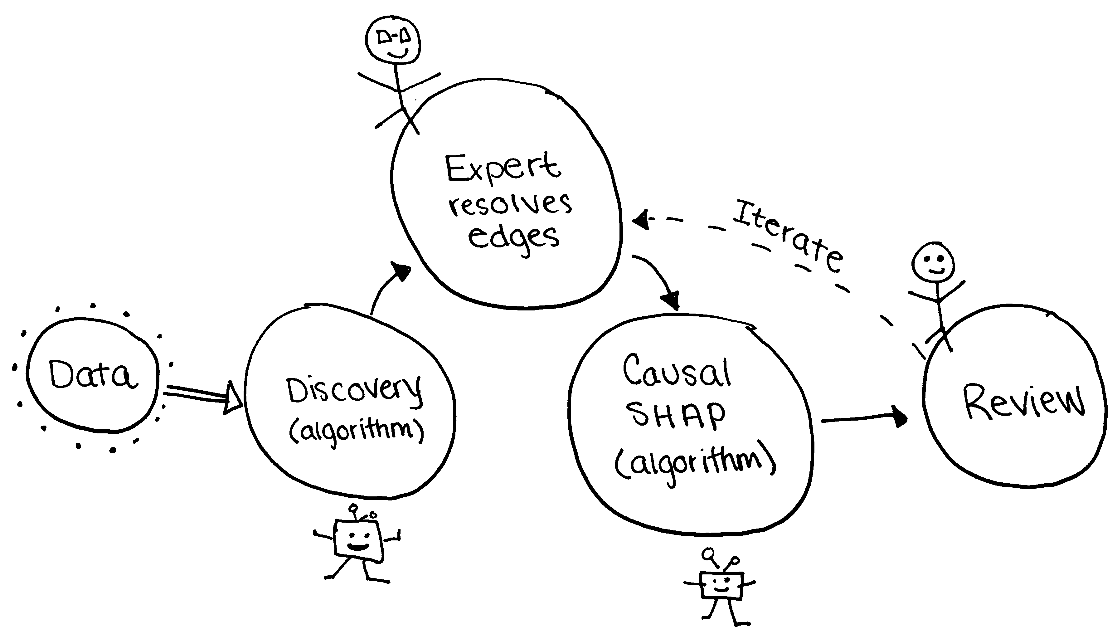
Without the cycle, each step is brittle. Causal discovery alone returns a CPDAG with ambiguous edges no statistical test can resolve. Causal SHAP alone needs a fully directed graph it cannot produce on its own. The expert in the middle, orienting the ambiguous edges using temporal logic and clinical knowledge, is what turns the CPDAG into something Causal SHAP can consume. The expert at the end, reading the attribution and deciding whether to flip an edge and run it again, is what makes the result defensible.
What we found
Standard SHAP averages over feature orderings as if they were exchangeable. Causal SHAP applied within an expert-augmented DAG workflow stops doing that, and the cost of that single change is modest. In the simcausal benchmark, where direct effects dominate, the two methods recovered the true causal ranking equally well. In the ICU pressure-injury setting, where confounding by indication and long mediator chains do most of the work, Causal SHAP demoted the treatment markers a clinician would have flagged as suspicious for good reason. The same workflow surfaced the upstream severity drivers that actually warrant intervention.
An alternative path: adjustment-set SHAP
A complementary approach sidesteps the permutation problem entirely. Use the DAG to identify a valid , the confounders that block all backdoor paths between treatment and outcome. Then fit a restricted prediction model using only those features and run vanilla SHAP on it. Because the feature set is restricted to confounders (no mediators, no , no descendants of treatment), the SHAP values cannot be contaminated by the topological artifact.
Adjustment-set SHAP is simpler and faster than DAG-constrained Shapley. It is also less granular: attribution for mediators is no longer available because the mediators are not in the model. We report it alongside the full Causal SHAP for cases where the question is purely about confounding-adjusted feature importance and the mediator decomposition is not needed.
Is this circular reasoning?
A natural objection deserves a direct answer: if we already know the DAG, why bother with SHAP at all? The objection assumes SHAP is producing causal answers that the DAG would then duplicate. It isn't. As we referenced earlier, standard SHAP decomposes a fitted model's predictions. That is a model-internal quantity, not a causal claim. Adding causal structure to it is not double-counting; it is bringing causal information into a method that has none.
The DAG and Causal SHAP are doing different work. The DAG is qualitative: it says “Treatment causes Inflammation” without saying by how much or for which fitted model. Causal SHAP is quantitative and model-specific: it decomposes a particular fitted model's prediction along the pathways the DAG permits. Two different models trained on the same data with the same DAG produce different Causal SHAP values, because they learn different functional relationships. The DAG redirects credit. It does not generate it.
In the 50-permutation simulation, adding DAG constraints moved the ranking—including Treatment—from the standard-SHAP result. That movement demonstrates that the structural assumptions matter, but it is not automatically an accuracy gain: at 500 permutations, both methods showed similar agreement with the benchmark. No one objects that a DAG can determine which variables to adjust for before a model estimates their associations. Causal SHAP follows the same division of labor: the DAG supplies structure, and the fitted model supplies model-specific attribution.
Closing thought
Feature importance methods assign credit, and credit is a causal question whether or not we treat it as one. When a fitted model is going to inform a clinical decision, the explanation it produces carries causal weight in practice even if the math behind it does not. Causal SHAP makes that math match the practice, and the cost of getting it right is one DAG that an expert can defend.
Future direction: sensing causal depth
A promising next step is to pair the DAG-resolved Causal SHAP workflow with Lucidity's Luma Warp technology. The early idea is not to ask another algorithm for a second feature-importance ranking. It is to ask whether the feature appears deeply entangled with the rest of the system in a way that may reveal causal depth or mediator-obscured signal.
The exploratory ELO-style score below should be read as a complexity signal: how nonlinear and interrelated a feature appears with the other inputs as those relationships pertain to the target. High ELO does not prove that a feature is important or causal. It points to features worth interrogating against the expert DAG, especially when ordinary attribution may have shifted credit toward downstream mediators.
Sneak peek: Luma Warp ELO diagnostic
| Rank | Feature | ELO |
|---|---|---|
| 1 | max_peep | 78 |
| 2 | max_temp_48h | 63 |
| 3 | min_O2_sat_48h | 61 |
| 4 | min_HR_48h | 61 |
| 5 | max_lactate_48h | 56 |
| 6 | lab_count_48h | 55 |
References
Active links to DOIs, arXiv records, and PubMed Central where available.
Foundational SHAP and interpretability
- 1.Shapley LS (1953). A value for n-person games. In Contributions to the Theory of Games, vol. 2, pp. 307–317. Princeton University Press.
- 2.Lundberg SM, Lee S-I (2017). A unified approach to interpreting model predictions. NeurIPS 30.ResearchGate
- 3.Rudin C (2019). Stop Explaining Black Box Machine Learning Models for High Stakes Decisions and Use Interpretable Models Instead. Nature Machine Intelligence 1:206–215.DOI: 10.1038/s42256-019-0048-xPubMed: 35603010
Causal SHAP methodology
- 4.Heskes T, Bucur IG, Claassen T (2020). Causal Shapley values: Exploiting causal knowledge to explain individual predictions of complex models. NeurIPS 33.arXiv:2011.01625
- 5.Janzing D, Minorics L, Blöbaum P (2020). Feature relevance quantification in explainable AI: A causal problem. AISTATS.arXiv:1910.13413
- 6.Frye C, Rowat C, Feige I (2020). Asymmetric Shapley values: Incorporating causal knowledge into model-agnostic explainability. NeurIPS 33.arXiv:1910.06358
- 7.Wang J, Wiens J, Lundberg S (2021). Shapley Flow: A graph-based approach to interpreting model predictions. AISTATS.arXiv:2010.14592
- 8.Ng WY, Wang LR, Liu S, Fan X (2025). Causal SHAP: Feature attribution with dependency awareness through causal discovery. IJCNN.arXiv:2509.00846
- 9.Koh H (in review). Principled feature importance and explanations for causal forests via Shapley values. R package shapcf.GitHub: hk1785/shapcf
Causal inference foundations
- 10.Pearl J (2009). Causality: Models, Reasoning, and Inference (2nd ed.). Cambridge University Press.
- 11.Spirtes P, Glymour C, Scheines R (2000). Causation, Prediction, and Search (2nd ed.). MIT Press.
- 12.Shrier I, Platt RW (2008). Reducing bias through directed acyclic graphs. BMC Medical Research Methodology 8:70.DOI: 10.1186/1471-2288-8-70PubMed: 18973665
- 13.VanderWeele TJ, Shpitser I (2011). A new criterion for confounder selection. Biometrics 67(4):1406–1413.DOI: 10.1111/j.1541-0420.2011.01619.x
- 14.Textor J, van der Zander B, Gilthorpe MS, Liśkiewicz M, Ellison GT (2016). Robust causal inference using directed acyclic graphs: The R package dagitty. International Journal of Epidemiology 45(6):1887–1894.DOI: 10.1093/ije/dyw341
Real-world data and simulation tooling
- 15.Johnson AEW et al. (2023). MIMIC-IV, a freely accessible electronic health record dataset. Scientific Data 10:1.DOI: 10.1038/s41597-022-01899-x
- 16.Alderden J et al. (2024). Explainable Artificial Intelligence for Early Prediction of Pressure Injury Risk. American Journal of Critical Care.
- 17.Sofrygin O, Neugebauer R, van der Laan MJ (2017). simcausal R Package: Conducting Transparent and Reproducible Simulation Studies of Causal Effect Estimation with Complex Longitudinal Data. Journal of Statistical Software 81(2):1–47.DOI: 10.18637/jss.v081.i02
XAI in life sciences and CDSSs
- 18.Abbas Q, Jeong W, Lee SW (2025). Explainable AI in Clinical Decision Support Systems: A Meta-Analysis of Methods, Applications, and Usability Challenges. Healthcare 13(17):2154.DOI: 10.3390/healthcare13172154PubMed: 40941506PMC: PMC12427955
- 19.El Arab RA et al. (2025). Artificial intelligence in hospital infection prevention: an integrative review. Frontiers in Public Health 13:1547450.DOI: 10.3389/fpubh.2025.1547450PubMed: 40241963
Cite this work
Harrison A, Pasi L, Ross J, Alderden JG, Wilson A (2026). Expert-Augmented Causal SHAP: Recovering DAG-Consistent Feature Importance via Iterative Causal Discovery and Domain Knowledge. ACIC 2026 Poster Session 2, Salt Lake City, May 13.
Corresponding contacts
The poster has five authors, listed with affiliations at the top of this page. For questions about the companion site, reach out to:
- Aimee Harrisonaimeewrightharrison@gmail.comLinkedIn
- Andy Wilsonwilson.stats@gmail.comLinkedIn